网址：https://ww2.mathworks.cn/help/signal/ug/cepstrum-analysis.html
描述：本案例由2个示例构成

-

-

针对以上案例，采用Python语言实现。

-

import matplotlib.pyplot as plt 
import numpy as np

倒频谱分析是一种非线性信号处理方法，在语音和图像处理等领域有多种应用。

序列 x 的复倒频谱是通过求 x 的傅里叶变换的复自然对数，然后对得到的序列进行傅里叶逆变换来计算的

$ \widehat{x} = \frac{1}{2\pi}\int_{-\pi}^{\pi}log[X(e^{j\omega})]e^{j\omega n}d\omega $

t = np.array(np.arange(0,1.28,0.01),dtype = complex)
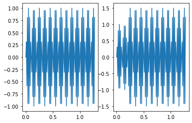
s1 = np.sin(2*np.math.pi*45*t)
s1.shape
s2 = s1+0.5*np.r_[np.zeros(20),s1[0:108]]

首先，创建以 100 Hz 采样的 45 Hz 正弦波。在信号开始 0.2 秒后，添加一个幅值减半的回声。

plt.subplot(1,2,1)
plt.plot(t,s1)
plt.subplot(1,2,2)
plt.plot(t,s2)

D:\anaconda\envs\pytorch\lib\site-packages\numpy\core\_asarray.py:83: ComplexWarning: Casting complex values to real discards the imaginary part
  return array(a, dtype, copy=False, order=order)
D:\anaconda\envs\pytorch\lib\site-packages\numpy\core\_asarray.py:83: ComplexWarning: Casting complex values to real discards the imaginary part
  return array(a, dtype, copy=False, order=order)





[<matplotlib.lines.Line2D at 0x17a010cb198>]

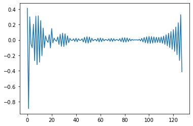
计算并绘制新信号的复倒频谱。

spectrum = np.fft.fft(s2)
ceps = np.fft.ifft(np.log(spectrum))

plt.plot(ceps)

D:\anaconda\envs\pytorch\lib\site-packages\numpy\core\_asarray.py:83: ComplexWarning: Casting complex values to real discards the imaginary part
  return array(a, dtype, copy=False, order=order)





[<matplotlib.lines.Line2D at 0x17a0120d240>]

-

对复倒频谱求逆

x = np.arange(1,11,1)
spectrum2 = np.fft.fft(x)
ceps2 = np.fft.ifft(np.log(spectrum2))
x

array([ 1,  2,  3,  4,  5,  6,  7,  8,  9, 10])

$ c_x = \frac{1}{2\pi}\int_{-\pi}^{\pi}log[X(e^{j\omega})]e^{j\omega n}d\omega $

cc = np.fft.fft(ceps2)
# cc = np.abs(cc)
cc2 = np.exp(cc)
cc3 = np.fft.ifft(cc2).real

cc3

array([ 1.,  2.,  3.,  4.,  5.,  6.,  7.,  8.,  9., 10.])