网址：https://ww2.mathworks.cn/help/signal/ug/analytic-signal-for-cosine.html
描述：本案例由1个示例构成

-

针对以上案例，采用Python语言实现。

-

本例展示了确定解析信号的方式，同时也演示了余弦信号对应的解析信号虚部是一个同频率的正弦信号。如果该余弦信号的均值非零（具有直流偏置），那么它的解析信号的实部是一个具有相同均值的余弦信号，但虚部的均值为零。

创建一个频率为100Hz的余弦信号，采样率为10kHz，并添加2.5的直流偏置。

import numpy as np
from scipy.signal import hilbert
import matplotlib.pyplot as plt
from mpl_toolkits.mplot3d import Axes3D
t = np.arange(0,1,1e-4)
x = 2.5 + np.cos(2*np.pi*100*t)

使用Hilbert函数来获取解析信号。解析信号的实部等于原信号，虚部是原信号的Hilbert变换。将实部与虚部绘制出来进行比较。

y = hilbert(x)
plt.plot(t,y.real)
plt.plot(t,y.imag)
plt.xlim([0,0.1])
plt.axis([0,0.1,-1,4])
plt.text(0.015,3.7,'Real Part \u2193')
plt.text(0.015,1.2,'Imaginary Part \u2193')

Text(0.015, 1.2, 'Imaginary Part ↓')

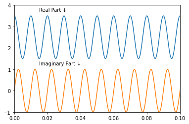
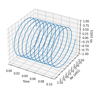
可以看到虚部是一个与实部具有相同频率的正弦信号，但虚部的均值为0，实部的均值为2.5。 原信号为 $$x(t)=2.5+cos(2π1000t)$$ 解析信号的结果为 $$z(t)=2.5+e^j2π1000t$$ 绘制10个周期的复数信号。

fig = plt.figure()
ax = Axes3D(fig)
prds = np.arange(1,1000,1)

ax.plot3D(t[prds],y.real[prds],y.imag[prds])
ax.set_xlabel('Time')
ax.set_ylabel('Re {z(t)}')
ax.set_zlabel('Im {z(t)}')

C:\Users\Lenovo\AppData\Local\Temp\ipykernel_5724\3629175957.py:2: MatplotlibDeprecationWarning: Axes3D(fig) adding itself to the figure is deprecated since 3.4. Pass the keyword argument auto_add_to_figure=False and use fig.add_axes(ax) to suppress this warning. The default value of auto_add_to_figure will change to False in mpl3.5 and True values will no longer work in 3.6.  This is consistent with other Axes classes.
  ax = Axes3D(fig)





Text(0.5, 0, 'Im {z(t)}')